Fizz Buzz with Cosines

Fizz Buzz is a children's word game that has become quite popular as a simple computer programming exercise. The game is simple. Players say the numbers aloud in order beginning with one. Whenever a number is divisible by \( 3, \) they say 'Fizz' instead. Whenever a number is divisible by \( 5, \) they say 'Buzz'. If a number is divisible by both \( 3 \) and \( 5, \) the player says both 'Fizz' and 'Buzz'. Here is a typical Python program that prints this sequence:

for n in range(1, 101):
    if n % 15 == 0:
        print('FizzBuzz')
    elif n % 3 == 0:
        print('Fizz')
    elif n % 5 == 0:
        print('Buzz')
    else:
        print(n)

Can we make it more complicated? Perhaps we can use trigonometric functions to encode all four cases in a single closed-form expression? That's what we are going to explore in this post. In fact, by the end of this post, we'll obtain a finite Fourier series that can take an input integer \( n \) and look up the text to be printed.

Contents

• Definitions
  • Symbol Functions
  • Fizz Buzz Sequence
• Indicator Functions
• Complex Exponentials
• Cosines
• Conclusion

Definitions

Before going any further, we establish a precise mathematical definition for the Fizz Buzz sequence. We begin by introducing a few functions that will help us define the Fizz Buzz sequence later.

Symbol Functions

We define a set of four functions \( \{ s_0, s_1, s_2, s_3 \} \) for integers \( n \) by: \begin{align*} s_0(n) &= n, \\ s_1(n) &= \mathtt{Fizz}, \\ s_2(n) &= \mathtt{Buzz}, \\ s_3(n) &= \mathtt{FizzBuzz}. \end{align*} We call these the symbol functions because they produce every term that appears in the Fizz Buzz sequence. The symbol function \( s_0 \) returns \( n \) itself. The functions \( s_1, \) \( s_2 \) and \( s_3 \) are constant functions that always return the literal words \( \mathtt{Fizz}, \) \( \mathtt{Buzz} \) and \( \mathtt{FizzBuzz} \) respectively, no matter what the value of \( n \) is.

Fizz Buzz Sequence

Now we can define the Fizz Buzz sequence as the sequence \[ (s_{f(n)}(n))_{n = 1}^{\infty} \] where \[ f(n) = \begin{cases} 1 & \text{if } n \equiv 0 \pmod{3} \text{ and } n \not\equiv 0 \pmod{5}, \\ 2 & \text{if } n \not\equiv 0 \pmod{3} \text{ and } n \equiv 0 \pmod{5}, \\ 3 & \text{if } n \equiv 0 \pmod{3} \text{ and } n \equiv 0 \pmod{5}, \\ 0 & \text{otherwise}. \end{cases} \] With this definition in place, we can expand the first few terms explicitly as follows: \begin{align*} (s_{f(n)}(n))_{n = 1}^{\infty} &= (s_{f(1)}(1), \; s_{f(2)}(2), \; s_{f(3)}(3), \; s_{f(4)}(4), \; s_{f(5)}(5), \; s_{f(6)}(6), \; s_{f(7)}(7), \; \dots) \\ &= (s_0(1), \; s_0(2), \; s_1(3), \; s_0(4), s_2(5), \; s_1(6), \; s_0(7), \; \dots) \\ &= (1, \; 2, \; \mathtt{Fizz}, \; 4, \; \mathtt{Buzz}, \; \mathtt{Fizz}, \; 7, \; \dots). \end{align*} Note how the function \( f(n) \) selects an index \( i \) that we then use to look up the symbol function \( s_i(n) \) which produces the \( n \)th term of the sequence.

Indicator Functions

In the previous section, we saw the function \[ f(n) = \begin{cases} 1 & \text{if } n \equiv 0 \pmod{3} \text{ and } n \not\equiv 0 \pmod{5}, \\ 2 & \text{if } n \not\equiv 0 \pmod{3} \text{ and } n \equiv 0 \pmod{5}, \\ 3 & \text{if } n \equiv 0 \pmod{3} \text{ and } n \equiv 0 \pmod{5}, \\ 0 & \text{otherwise}. \end{cases} \] which helps us to select a function \( s_{f(n)}(n) \) which in turn determines the \( n \)th term of the Fizz Buzz sequence.

Our goal now is to replace this piecewise formula with a single closed-form expression. To do so, we first define indicator functions \( I_m(n) \) as follows: \[ I_m(n) = \begin{cases} 1 & \text{if } n \equiv 0 \pmod{m}, \\ 0 & \text{if } n \not\equiv 0 \pmod{m}. \end{cases} \] The formula for \( f(n) \) can now be written as: \[ f(n) = \begin{cases} 1 & \text{if } I_3(n) = 1 \text{ and } I_5(n) = 0, \\ 2 & \text{if } I_3(n) = 0 \text{ and } I_5(n) = 1, \\ 3 & \text{if } I_3(n) = 1 \text{ and } I_5(n) = 1, \\ 0 & \text{if } I_3(n) = 0 \text{ and } I_5(n) = 0. \end{cases} \] Let us reorder the cases and conditions to see if any pattern emerges. \[ f(n) = \begin{cases} 0 & \text{if } I_5(n) = 0 \text{ and } I_3(n) = 0, \\ 1 & \text{if } I_5(n) = 0 \text{ and } I_3(n) = 1, \\ 2 & \text{if } I_5(n) = 1 \text{ and } I_3(n) = 0, \\ 3 & \text{if } I_5(n) = 1 \text{ and } I_3(n) = 1. \end{cases} \] Do you see the pattern? Here is the same function written as a table:

Do you see it now? If we treat the values in the first two columns as binary digits (bits) and the values in the third column as decimal numbers, then in each row the first two columns give the binary representation of the number in the third column. For example, \( 3_{10} = 11_2 \) and indeed in the last row of the table, we see the bits \( 1 \) and \( 1 \) in the first two columns and the number \( 3 \) in the last column. In other words, if we treat the values of \( I_5(n) \) and \( I_3(n) \) as bits, then \[ (f(n))_{10} = \left( I_5(n) I_3(n) \right)_2. \] Therefore \[ f(n) = 2 \, I_5(n) + I_3(n). \] We can now write a small program to demonstrate this formula:

for n in range(1, 101):
    s = [n, 'Fizz', 'Buzz', 'FizzBuzz']
    i = (n % 3 == 0) + 2 * (n % 5 == 0)
    print(s[i])

We can make it even shorter at the cost of some clarity:

for n in range(1, 101):
    print([n, 'Fizz', 'Buzz', 'FizzBuzz'][(n % 3 == 0) + 2 * (n % 5 == 0)])

What we have obtained so far is pretty good. While there is no universal definition of a closed-form expression, I think most people would agree that the indicator functions as defined above are simple enough to be permitted in a closed-form expression.

Complex Exponentials

In the previous section, we obtained the formula \[ f(n) = I_3(n) + 2 \, I_5(n) \] which we then used as an index to look up the text to be printed. We also argued that this is a pretty good closed-form expression already.

However, in the interest of making things more complicated, we must ask ourselves: What if we are not allowed to use the indicator functions? What if we must adhere to the commonly accepted meaning of a closed-form expression which allows only finite combinations of basic operations such as addition, subtraction, multiplication, division, integer exponents and roots with integer index as well as functions such as exponentials, logarithms and trigonometric functions. It turns out that the above formula can be rewritten using only addition, multiplication, division and the cosine function. Let us begin the translation.

Consider the sum \[ S_m(n) = \sum_{k = 0}^{m - 1} e^{2 \pi i k n / m}, \] where \( i \) is the imaginary unit and \( n \) and \( m \) are integers. This is a geometric series in the complex plane with ratio \( r = e^{2 \pi i n / m}. \) If \( n \) is a multiple of \( m , \) then \( n = cm \) for some integer \( c \) and we get \[ r = e^{2 \pi i n / m} = e^{2 \pi i c} = 1. \] Therefore, when \( n \) is a multiple of \( m, \) we get \[ S_m(n) = \sum_{k = 0}^{m - 1} 1 = m. \] If \( n \) is not a multiple of \( m, \) then \( r \ne 1 \) and the geometric series becomes \[ S_m(n) = \frac{r^m - 1}{r - 1} = \frac{e^{2 \pi i n} - 1}{e^{2 \pi i n / m} - 1} = 0. \] Therefore, \[ S_m(n) = \begin{cases} m & \text{if } n \equiv 0 \pmod{m}, \\ 0 & \text{if } n \not\equiv 0 \pmod{m}. \end{cases} \] Dividing both sides by \( m, \) we get \[ \frac{S_m(n)}{m} = \begin{cases} 1 & \text{if } n \equiv 0 \pmod{m}, \\ 0 & \text{if } n \not\equiv 0 \pmod{m}. \end{cases} \] But the right-hand side is \( I_m(n). \) Therefore \[ I_m(n) = \frac{S_m(n)}{m} = \frac{1}{m} \sum_{k = 0}^{m - 1} e^{2 \pi i k n / m}. \]

Cosines

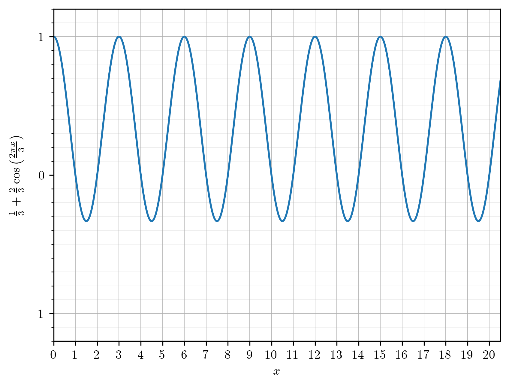
We begin with Euler's formula \[ e^{i x} = \cos x + i \sin x \] where \( x \) is a real number. From this formula, we get \[ e^{i x} + e^{-i x} = 2 \cos x. \] Therefore \begin{align*} I_3(n) &= \frac{1}{3} \sum_{k = 0}^2 e^{2 \pi i k n / 3} \\ &= \frac{1}{3} \left( 1 + e^{2 \pi i n / 3} + e^{4 \pi i n / 3} \right) \\ &= \frac{1}{3} \left( 1 + e^{2 \pi i n / 3} + e^{-2 \pi i n / 3} \right) \\ &= \frac{1}{3} + \frac{2}{3} \cos \left( \frac{2 \pi n}{3} \right). \end{align*} The third equality above follows from the fact that \( e^{4 \pi i n / 3} = e^{6 \pi i n / 3} e^{-2 \pi i n / 3} = e^{2 \pi i n} e^{-2 \pi i n/3} = e^{-2 \pi i n / 3}. \)

The function above is defined for integer values of \( n \) but we can extend its formula to real \( x \) and plot it to observe its shape between integers. As expected, the function takes the value \( 1 \) whenever \( x \) is an integer multiple of \( 3 \) and \( 0 \) whenever \( x \) is an integer not divisible by \( 3. \)

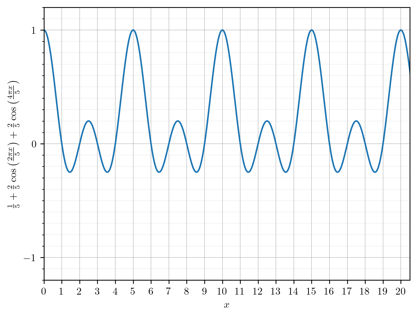
Similarly, \begin{align*} I_5(n) &= \frac{1}{5} \sum_{k = 0}^4 e^{2 \pi i k n / 5} \\ &= \frac{1}{5} \left( 1 + e^{2 \pi i n / 5} + e^{4 \pi i n / 5} + e^{6 \pi i n / 5} + e^{8 \pi i n / 5} \right) \\ &= \frac{1}{5} \left( 1 + e^{2 \pi i n / 5} + e^{4 \pi i n / 5} + e^{-4 \pi i n / 5} + e^{-2 \pi i n / 5} \right) \\ &= \frac{1}{5} + \frac{2}{5} \cos \left( \frac{2 \pi n}{5} \right) + \frac{2}{5} \cos \left( \frac{4 \pi n}{5} \right). \end{align*} Extending this expression to real values of \( x \) allows us to plot its shape as well. Once again, the function takes the value \( 1 \) at integer multiples of \( 5 \) and \( 0 \) at integers not divisible by \( 5. \)

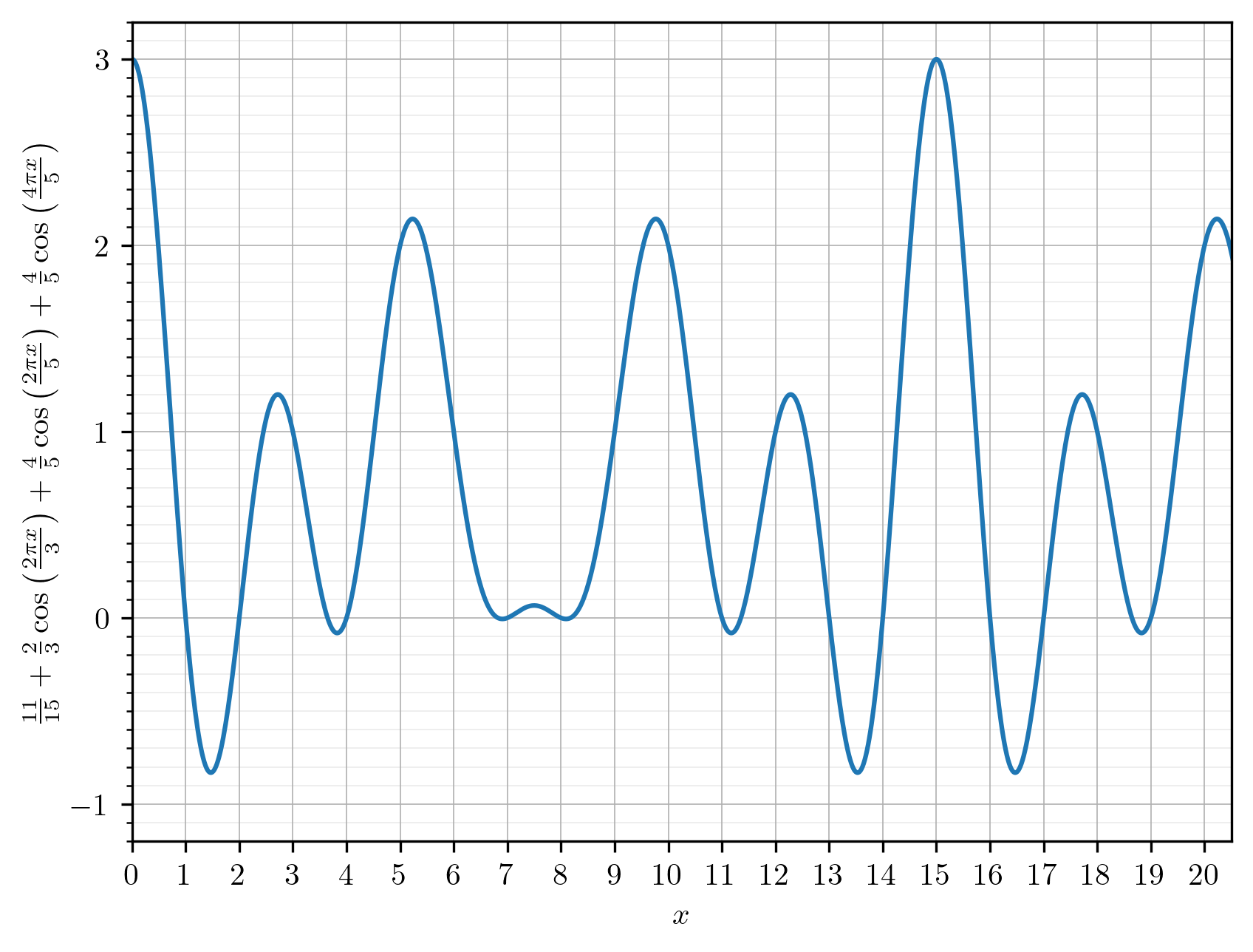
Recall that we expressed \( f(n) \) as \[ f(n) = I_3(n) + 2 \, I_5(n). \] Substituting these trigonometric expressions yields \[ f(n) = \frac{1}{3} + \frac{2}{3} \cos \left( \frac{2 \pi n}{3} \right) + 2 \cdot \left( \frac{1}{5} + \frac{2}{5} \cos \left( \frac{2 \pi n}{5} \right) + \frac{2}{5} \cos \left( \frac{4 \pi n}{5} \right) \right). \] A straightforward simplification gives \[ f(n) = \frac{11}{15} + \frac{2}{3} \cos \left( \frac{2 \pi n}{3} \right) + \frac{4}{5} \cos \left( \frac{2 \pi n}{5} \right) + \frac{4}{5} \cos \left( \frac{4 \pi n}{5} \right). \] We can extend this expression to real \( x \) and plot it as well. The resulting curve takes the values \( 0, 1, 2 \) and \( 3 \) at integer points, as desired.

Now we can write our Python program as follows:

from math import cos, pi
for n in range(1, 101):
    s = [n, 'Fizz', 'Buzz', 'FizzBuzz']
    i = round(11 / 15 + (2 / 3) * cos(2 * pi * n / 3)
                      + (4 / 5) * cos(2 * pi * n / 5)
                      + (4 / 5) * cos(4 * pi * n / 5))
    print(s[i])

Conclusion

To summarise, we have defined the Fizz Buzz sequence as \[ (s_{f(n)}(n))_{n = 1}^{\infty} \] where \[ f(n) = \frac{11}{15} + \frac{2}{3} \cos \left( \frac{2 \pi n}{3} \right) + \frac{4}{5} \cos \left( \frac{2 \pi n}{5} \right) + \frac{4}{5} \cos \left( \frac{4 \pi n}{5} \right) \in \{ 0, 1, 2, 3 \} \] and \( s_0(n) = n, \) \( s_1(n) = \mathtt{Fizz}, \) \( s_2(n) = \mathtt{Buzz} \) and \( s_3(n) = \mathtt{FizzBuzz}. \) A Python program to print the Fizz Buzz sequence based on this definition was presented earlier. That program can be written more succinctly as follows:

from math import cos, pi
for n in range(1, 101):
    print([n, 'Fizz', 'Buzz', 'FizzBuzz'][round(11 / 15 + (2 / 3) * cos(2 * pi * n / 3) + (4 / 5) * (cos(2 * pi * n / 5) + cos(4 * pi * n / 5)))])

The keen-eyed might notice that the expression we have obtained for \( f(n) \) is a finite Fourier series. This is not surprising, since the output of a Fizz Buzz program depends only on \( n \bmod 15. \) Any function on a finite cyclic group can be written exactly as a finite Fourier expansion.

We have taken a simple counting game and turned it into a trigonometric construction: a finite Fourier series with a constant term \( 11/15 \) and three cosine terms with coefficients \( 2/3, \) \( 4/5 \) and \( 4/5. \) None of this makes Fizz Buzz any easier, of course, but it does mean that every \( \mathtt{Fizz} \) and \( \mathtt{Buzz} \) now owes its existence to its Fourier coefficients. We began with the modest goal of making this simple problem more complicated. I think it is safe to say that we have not fallen short.